Marketing Mix Modelling Comes Back
A 1960s regression became the post-privacy measurement of record. How MMM actually works, what adstock and saturation are doing, why it must be calibrated against experiments, and the failure modes that make a model confidently wrong.
Assumed knowledge
On this page
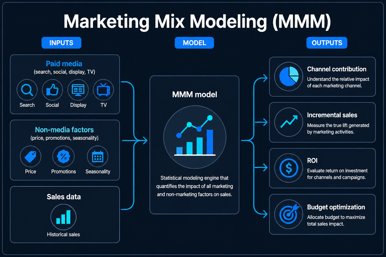
Marketing mix modelling is a regression. You take a few years of weekly sales, a few years of weekly spend by channel, everything else that moved sales — price, promotions, distribution, weather, competitors, Christmas — and you fit a model that assigns a share of the outcome to each input.
That is it. No cookies, no device graph, no user-level log. It was doing this in packaged goods in the 1960s, it was unfashionable for the entire decade when click tracking seemed to answer the question for free, and it came back because that decade ended.
Why it came back
Three things happened at once.
The identifiers went away. Safari and Firefox blocked years ago, iOS 14.5 made the IDFA opt-in, and while Chrome kept its cookies in the end — see Life After Third-Party Cookies — the signal that user-level depended on was already gone for a large share of traffic. MMM never needed that signal, because it never looks at a user.
The walled gardens stopped being measurable from outside. Much of the biggest spend now sits inside platforms that will report on themselves and will not export the logs you would need to check. MMM treats each one as a column of spend and judges it by what happened to total sales, which is the one question a self-reported dashboard cannot answer.
The channels stopped being clickable. CTV, audio, retail media in-store, DOOH. Half the growth in media is in formats where there is no click to attribute, so a measurement method whose unit of analysis is the click has nothing to say about them.
The two curves that make it a model
A straight regression of sales on spend would be useless, because advertising does not behave linearly in either time or volume. Two transformations fix that, and they are where most of the modelling actually lives.
Adstock: advertising persists
An impression today affects sales next week. Adstock — Simon Broadbent's formulation — carries a fraction of each period's effect into the next:
adstock(t) = spend(t) + λ · adstock(t − 1)λ is the decay rate. At λ = 0.5, half the effect survives each week, so a burst still has a quarter of its force two weeks later and an eighth three weeks later. Brand video typically fits a long decay; a promotional email fits almost none. Many implementations add a delay term as well, because a TV campaign often peaks a week or two after the flight rather than during it.
Get λ wrong and the model misreads the calendar: too short and you credit the sales to whatever ran later, too long and you credit a channel for sales it had nothing to do with.
Saturation: the tenth million is not the first
Doubling spend does not double response. The relationship is concave — usually fitted with a Hill function or a negative-exponential curve — and that curve is the output people actually use.
What comes out
Four things, in descending order of how much you should trust them.
| Output | What it is | Trust |
|---|---|---|
| Channel contribution | Share of sales attributed to each channel plus a baseline | Moderate — sensitive to specification |
| Marginal return / saturation curve | What the next dollar in each channel does | Moderate, and the most useful thing in the model |
| ROI per channel | Contribution divided by spend | Low on its own, routinely over-read |
| Optimised budget | The allocation that maximises modelled sales | Only as good as the curves beneath it |
The baseline deserves attention. It is the sales you would have made with no advertising at all — brand equity, distribution, habit — and it is usually the largest single term. Models that fit an implausibly large baseline are quietly saying "advertising does very little", and models that fit a small one are often absorbing a trend into the media coefficients. Ask what the baseline is before you ask what the ROI is.
Bayesian, because the data is thin
The modern tooling — Google's Meridian, Meta's Robyn, PyMC-Marketing — is mostly Bayesian, and that is a response to a real problem rather than a fashion.
Three years of weekly data is 156 observations. With ten channels, adstock and saturation parameters each, plus price, promotions, seasonality and a trend, you have more parameters than you can responsibly fit. Worse, media spends move together: budgets go up in Q4 for everything at once, which makes the regression unable to tell channels apart. That is multicollinearity, and in a frequentist fit it shows up as coefficients that swing wildly — sometimes negative — for no substantive reason.
A Bayesian model handles this by requiring you to state what you already believe. Priors on each channel's effectiveness, on decay, on the shape of saturation. The output is a distribution rather than a point, so the honest answer becomes "this channel's ROI is somewhere between 1.8 and 4.1" instead of a single number with three decimal places and no error bar.
Calibration: the part people skip
A regression finds correlation. Nothing in the maths makes a coefficient causal, and the standard failure is a channel that targets people who were already going to buy — brand search, retargeting — absorbing credit for the purchases it merely accompanied. This is the harvesting trap from The Marketing Funnel appearing again, one level up.
The fix is to pin the model to something that is causal. Run geo holdout experiments on a few channels, measure the lift directly, and use those measured effects as priors — or as hard constraints — in the model. Google's and Meta's documentation both treat experiment calibration as a requirement rather than an enhancement, and uncalibrated channel-level ROIs routinely sit well outside the experimental estimate.
The practical arrangement, often called triangulation:
- Experiments answer "did this specific thing work?" with the most credibility and the least coverage. See Incrementality: the Only Honest Number.
- MMM answers "how should the whole budget be split?" across everything, including unclickable media, with moderate credibility.
- Attribution answers "what happened in-flight?" fast and daily, with the least credibility. See Every Attribution Model Is Wrong.
Use each for what it is good at. Where MMM and an experiment disagree, the experiment wins and the model gets recalibrated.
Failure modes
The ways a model becomes confidently wrong, roughly by frequency.
No variance to learn from. If a channel has run at the same weekly spend for two years, the model cannot tell you what changing it would do, because nothing ever changed. Always-on, flat budgets produce unidentifiable coefficients. Deliberately varying spend — flighting, regional differences, planned dark weeks — is what makes a channel measurable at all.
Collinearity between channels. Everything rising together in Q4 means the model attributes on the strength of a prior rather than on evidence.
Seasonality eating the media effect. Advertising peaks when demand peaks. A model with weak seasonality controls credits Christmas to the Christmas campaign.
Aggregation hiding everything. National weekly data cannot see that a channel works in one region and not another. Geo-level or product-level models have far more observations and are strictly better where the data exists.
Overfitting to the holdout. Tuning adstock and saturation until the out-of-sample fit looks good produces a model that predicts last year beautifully and allocates next year badly. Fit quality and decision quality are different objectives, and R² is not evidence of causality.
Refresh cadence treated as reporting. MMM is quarterly at best; the parameters simply do not move weekly. Teams that rebuild it monthly end up chasing noise and renegotiating budgets against it.
What it costs to run
Not the licence — the inputs. Two to three years of weekly history, spend by channel reconciled to what was actually delivered rather than what was planned, price and promotion calendars, distribution data, and someone able to defend a prior in a meeting. Most failed MMM projects fail at data assembly, and the most common single cause is media spend that cannot be reconciled with the finance system.
Check yourself
An MMM reports brand search at a 12:1 ROI — the highest of any channel. A geo holdout on the same channel measures an incremental 1.4:1. What should you conclude?
Key takeaways
- MMM regresses aggregate outcomes on media spend plus non-media drivers. It needs no user-level data, which is why the privacy decade brought it back.
- Adstock models persistence across time; saturation models diminishing returns within a period. The saturation curve, not the average ROI, is what should drive budget decisions.
- Modern MMM is Bayesian because 156 weekly observations cannot identify that many parameters. Priors are therefore part of the result — demand to see them.
- An uncalibrated model finds correlation and will hand credit to demand-harvesting channels. Calibrate against geo holdouts; where the two disagree, the experiment wins.
- A channel whose spend never varies cannot be measured. Varying budgets deliberately is what makes the model identifiable.
- Triangulate: experiments for credibility, MMM for allocation, attribution for speed. No single method covers all three.
Next
Incrementality: the Only Honest Number is the experimental half of this pair — how geo holdouts, ghost ads and PSA tests are designed, and why a measured lift usually lands well below the reported one.